| Issue |
Security and Safety
Volume 4, 2025
Security and Safety for Next Generation Industrial Systems
|
|
|---|---|---|
| Article Number | 2025007 | |
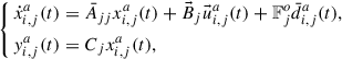
| Number of page(s) | 16 | |
| Section | Industrial Control | |
| DOI | https://doi.org/10.1051/sands/2025007 | |
| Published online | 25 October 2025 | |
Research Article
Countermeasures against collusive stealthy attacks in cyber-physical microgrids: A dynamic encoding approach
1
School of Mechatronic Engineering and Automation, Shanghai Key Laboratory of Power Station Automation Technology, Shanghai University, Shanghai, 200444, China
2
School of Optical-Electrical and Computer Engineering, University of Shanghai for Science and Technology, Shanghai, 200093, China
* Corresponding authors (email: This email address is being protected from spambots. You need JavaScript enabled to view it.
)
Received:
25
March
2025
Revised:
6
May
2025
Accepted:
8
July
2025
Abstract
Cyber-physical microgrids, as a representative industrial system, seamlessly integrate computation, communication, control, and physical devices, making it vulnerable to cyber-attacks that can trigger cascading failures and potentially lead to the collapse of the entire grid. This paper aims to develop an efficient detection framework for collusive stealthy attacks in cyber-physical microgrids. First, an ℒ∞ unknown input observer (UIO) is deployed at the control center to monitor communication links between distributed generation units (DGUs). By treating interconnections and secondary control as unknown inputs, the observer gain is designed using only local information. Then, the vulnerability of the ℒ∞ UIO-based monitoring unit is analyzed, and a collusive stealthy attack is devised to disrupt grid operations without alerting the ℒ∞ UIO-based detection mechanism. To counteract the novel attack, a dynamic encoding mechanism is developed for the communication links between DGUs. This mechanism involves encoding control signals prior to transmission and subsequently decoding them at the control center. Furthermore, an in-depth analysis of the feasibility criteria for the encoding matrix has been conducted. Eventually, the efficacy of the proposed detection framework is validated through a series of simulation experiments.
Key words: Cyber-physical microgrids / Stealthy attacks / Attack detection / Unknown input observer
Citation: Wu Z, Peng C, Tian E and Zhang Y. Countermeasures against collusive stealthy attacks in cyber-physical microgrids: A dynamic encoding approach. Security and Safety 2025; 4: 2025007. https://doi.org/10.1051/sands/2025007
© The Author(s) 2025. Published by EDP Sciences and China Science Publishing & Media Ltd.
 This is an Open Access article distributed under the terms of the Creative Commons Attribution License (https://creativecommons.org/licenses/by/4.0), which permits unrestricted use, distribution, and reproduction in any medium, provided the original work is properly cited.
1. Introduction
The evolution of industrial cyber-physical system (ICPS) marks a paradigm shift in engineering infrastructure, propelled by the synergistic integration of computational intelligence, control theory, and advanced communication paradigms [1]. Architecturally, these systems are hierarchically organized into three functional layers: the physical layer, encompassing operational entities ranging from power generation facilities to autonomous maritime systems; the application layer, which includes cyber systems such as supervisory control and data acquisition systems for information processing and decision-making; and the communication layer, which orchestrates the bidirectional flow of operational data and control directives. This interconnected architecture establishes a robust framework for seamless interaction between physical processes and cyber-based decision-making mechanisms. As a class of advanced systems, ICPS embodies structural complexity that necessitates interdisciplinary knowledge fusion across heterogeneous domains [2].
The integration of cutting-edge communication technologies has substantially increased the capabilities of cyber systems in achieving accurate data collection and optimizing decision-making processes, thus markedly increasing the operational efficiency of ICPS. Owing to their profound benefits, ICPS is increasingly recognized as a fundamental cornerstone in advancing critical infrastructure, fostering smart manufacturing initiatives, and driving the transition toward a green economy, among other pivotal applications. In summary, ICPS represents a key technological cornerstone of Industry 5.0, serving as an essential enabler to realize its overarching vision [3]. To date, ICPS has demonstrated extensive applicability across diverse domains, including healthcare and medical technologies, smart grid infrastructure, and intelligent transportation networks. These implementations have not only significantly enhanced quality of life but have also generated substantial economic value across multiple sectors. Among these applications, cyber-physical microgrids, as a paradigmatic example of ICPS, have garnered significant attention from both industrial and academic communities due to their capability to flexibly integrate various renewable energy sources, thereby substantially reducing carbon emissions [4].
The widespread implementation of open communication architectures in cyber-physical microgrid systems has been predominantly motivated by their operational efficiency and cost-effectiveness. Nevertheless, despite offering substantial economic benefits and enhanced deployment scalability, these public networks fundamentally expose critical infrastructure to advanced cyber vulnerabilities. Contemporary research [5–7] has documented a significant surge in cyber-security incidents targeting ICPS, with particular emphasis on cyber-physical DC microgrid, raising substantial concerns regarding societal resilience and infrastructure security [4]. When compared to their AC counterparts, DC microgrids demonstrate superior performance in power transmission efficiency while requiring lower investment in metering infrastructure and control units. This emerging threat landscape has been vividly illustrated through numerous critical infrastructure compromises of notable significance. In 2015, a sophisticated coordinated attack compromised Ukraine’s power grid, causing widespread blackouts and substantial infrastructure damage [8]. The following year witnessed the successful infiltration of a 200 MW generation facility in Kiev, resulting in its complete operational disruption [9]. More recently, in 2020, Venezuela’s national grid experienced a targeted assault on 765 trunk lines, affecting power supply across multiple regions. These consecutive security breaches highlight the imperative for implementing a defense strategy to ensure the operational continuity of cyber-physical microgrids.
Denial-of-Service (DoS) attacks primarily degrade network performance by drastically diminishing packet acceptance rates [10]. In contrast, false data injection (FDI) attacks pose a more intricate threat to data integrity through advanced manipulation techniques [11], rendering them inherently more difficult to detect. Building upon existing classical attack strategies, a variety of intelligent attack schemes have been successively proposed. For instance, in [12], an optimal DoS attack scheduling was designed to maximize the disruption of remote estimator performance. In [13], a critical data-based attack strategy combined with a stochastic energy allocation scheme was developed to degrade system performance. Beyond DoS attacks, more covert FDI attacks have also been constructed. For example, in [6], a dynamic feedback-based method was employed to design an optimal FDI attack aimed at maximizing output error. In [14], a zero-trace stealth attack was devised to compromise the operation of DC microgrids.
Currently, detection methodologies for FDI attacks can be fundamentally classified into two paradigms: analytical model-dependent solutions and data-driven learning methodologies. For instance, Euclidean distance was employed as a metric to quantify the variation in voltage signals and combined with pre-designed thresholds to detect attacks [15]. In [16], an interval observer was tailored for smart grid, capable of generating both upper and lower bounds for state estimation, and then determining whether an attack occurs based on whether the true state is within these bounds. In [17], a summation-based detector was proposed to identify FDI attacks, leveraging historical information to significantly enhance detection accuracy. Unlike the aforementioned model-based detection schemes, which rely on precise system models, the core concept of data-driven learning approaches lies in leveraging collected data to uncover underlying patterns and construct a detection model capable of distinguishing between normal and anomalous data. Specifically, in [18], a distributed support vector machine was implemented to detect stealthy FDI attacks in smart grids, employing principal component analysis for dimensionality reduction to mitigate computational complexity. In [19], a semi-supervised learning algorithm rooted in generative adversarial networks was utilized to train the model and infer the data distribution from samples, thereby distinguishing between attacked and normal states in the smart grid. Based on the aforementioned analysis, existing detection strategies may fail when confronted with coordinated attack tactics and struggle to adapt to the dynamic insertion or removal of subsystems.
This paper aims to construct an effective detection framework targeting collusive stealthy attacks in cyber-physical microgrids, with the following key contributions: (1) an ℒ∞ unknown input observer (UIO) is established at the control center to monitor DGU communication links relying solely on local data; (2) systematic analysis of UIO vulnerability enables the design of collusive stealthy attacks that disrupt microgrid operations while evading detection by the ℒ∞ UIO-based detection mechanism. Unlike conventional unobservable attacks [20], the proposed attack strategy conceals the attack signal as an unknown input and implements it in a collaborative manner; (3) dynamic encoding embedded within DGUs communication channels are proposed to expose the collusive stealthy attack, with geometric control theory deriving feasibility conditions for the encoding matrix.
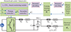 |
Figure 1. The overall architecture diagram of cyber-physical microgrid |
2. Model of cyber-physical microgrids
This article investigates a cyber-physical microgrid encompassing M interconnected distributed generation units (DGUs), as shown in Figure 1. Each DGU is equipped with a DC voltage source, an RLC filter, a local controller, a load, and a buck converter. The physical power network of microgrids can be represented as a weighted undirected connected graph 𝒢p = (𝒱p, ℰp, 𝒲p). In this graph, the vertex set 𝒱p = {1, 2, …, M} stands for DGUs. The edge set ℰp ⊆ 𝒱p × 𝒱p signifies the distribution lines that connect neighboring DGUs. The adjacency matrix ![Mathematical equation: $ {\mathscr{W}^{p}}=[w^{p}_{ij}]_{M\times M} $](/articles/sands/full_html/2025/01/sands20250008/sands20250008-eq1.gif) has nonnegative elements
has nonnegative elements  (∀(i, j)∈ℰp). Let 𝒩i
p = {j ∈ 𝒱p|(i, j)∈ℰp} denote the set of coupled neighboring units for DGU i. Moreover, the communication topology of the cyber layer, denoted as 𝒢c = (𝒱c, ℰc, 𝒲c), shares identical structural configuration and edge weight assignments with graph 𝒢p.
(∀(i, j)∈ℰp). Let 𝒩i
p = {j ∈ 𝒱p|(i, j)∈ℰp} denote the set of coupled neighboring units for DGU i. Moreover, the communication topology of the cyber layer, denoted as 𝒢c = (𝒱c, ℰc, 𝒲c), shares identical structural configuration and edge weight assignments with graph 𝒢p.
The dynamic behavior of DGU i is governed by the following differential equations derived through the systematic application of Kirchhoff’s voltage and current laws:
 (1)
(1)
where I ti(t), L ti, C ti, and R ti denote the current, inductance, capacitance, and resistance, respectively. V i(t) and V ti(t) correspond to the voltage at the ith point of common coupling (PCC) and the output voltage of the ith buck converter. As for the current flowing through the distribution line ij, modeled as an RL network, it is represented by I ij(t) and satisfies:
 (2)
(2)
where L
ij and R
ij respectively indicate the distribution line ij’s inductance and resistance. In Equation (2), the current I
ij(t) can be approximately regarded as  when assuming the quasi-static linear approximation, with V
j(t) denoting the voltage of the jth PCC.
when assuming the quasi-static linear approximation, with V
j(t) denoting the voltage of the jth PCC.
Figure 1 depicts that each DGU is equipped with a local primary controller, ensuring the voltage V
i(t) at the PCC follows the desired reference voltage  . To enhance voltage tracking precision, an integral compensation component is embedded in the DGU architecture, expressed mathematically as:
 (3)
(3)
where  denotes the voltage tracking error, v
i(t) corresponds to its integral term, and
denotes the voltage tracking error, v
i(t) corresponds to its integral term, and  defines the secondary control input, aimed at achieving voltage balancing and current sharing. Thus, the augmented dynamical model for DGU i is formulated as:
 (4)
(4)
where x i(t)=[V i(t),I ti(t),v i(t)]T ∈ ℝ3 stands for the state, y i(t)∈ℝ3 represents the measurement output, C i ∈ ℝ3 × 3 is identity matrix, other associated matrices are derived as follows:
![Mathematical equation: $$ \begin{aligned} \begin{aligned} A_{ii} =\left[ \begin{array}{ccc} 0&\frac{1}{C_{ti}}&0 \\ [4pt] -\frac{1}{L_{ti}}&-\frac{R_{ti}}{L_{ti}}&0 \\ -1&0&0 \\ \end{array} \right], A_{ij} =\left[ \begin{array}{ccc} \frac{1}{C_{ti}R_{ij}}&0&0\\ 0&0&0 \\ 0&0&0 \end{array} \right], \tilde{B}_{i} =\left[ \begin{array}{c} 0 \\ \frac{1}{L_{ti}} \\ 0 \\ \end{array} \right], \bar{B}_{i} =\left[ \begin{array}{c} 0 \\ 0 \\ 1 \\ \end{array} \right], \vec{B}_{i} =\left[ \begin{array}{cc} - \frac{1}{C_{ti}}&0\\ 0&0\\ 0&1\\ \end{array} \right]. \end{aligned} \end{aligned} $$](/articles/sands/full_html/2025/01/sands20250008/sands20250008-eq11.gif)
Furthermore, ![Mathematical equation: $ \vec{u}_{i}(t)=[I_{li}(t),V_{i}^{re}(t)]^T \in \mathbb{R}^{2} $](/articles/sands/full_html/2025/01/sands20250008/sands20250008-eq12.gif) represents the exogenous input, while
represents the exogenous input, while 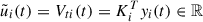 is the primary control input with K
i ∈ ℝ3 denoting the vector of primary control gains. A consensus-based coordination protocol is implemented to synthesize the secondary control signal
is the primary control input with K
i ∈ ℝ3 denoting the vector of primary control gains. A consensus-based coordination protocol is implemented to synthesize the secondary control signal  , governed by
![Mathematical equation: $$ \begin{aligned} \dot{\bar{u}}_{i}(t) = [0,k_i,0]\sum _{j \in \fancyscript {N}_i^{c}}{w_{ij}^c\left(\frac{y_{i}(t)}{I_{ti}^{s}}-\frac{y_{i,j}(t)}{I_{tj}^{s}}\right)}, \end{aligned} $$](/articles/sands/full_html/2025/01/sands20250008/sands20250008-eq15.gif) (5)
(5)
where k
i > 0 represents weight parameter,  and
and  represent current proportional parameters for DGU i and DGU j, y
i, j(t) represents the output of DGU j transmitted to DGU i. Without loss of generality, assume that the disturbance
represent current proportional parameters for DGU i and DGU j, y
i, j(t) represents the output of DGU j transmitted to DGU i. Without loss of generality, assume that the disturbance  , measurement noise
  , and
, and  are amplitude bounded, i.e.,
  ,
,  , and
, and 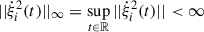 , where ||⋆||∞ and ||⋆|| represents the ℒ∞ norm and Euclidean norm, respectively.
3. Collusive stealthy attack mechanism
In light of the vulnerabilities, large-scale characteristics, and inherent uncertainties of cyber-physical microgrids, this section presents a detection scheme based on the ℒ∞ UIO for identifying communication link risks between DGUs. Additionally, a novel of collusive stealthy attack is proposed to bypass current defense mechanisms.
3.1. ℒ∞ UIO-based countermeasure
As illustrated in Figure 1 and the consensus scheme Equation (5), the secondary control of DGU i requires the measured outputs transmitted from neighboring DGU j. Malicious adversaries could exploit inherent vulnerabilities in communication channels to execute cyber intrusions, deliberately falsifying transmitted data and compromising information integrity. This adversarial manipulation directly impacts secondary control inputs, ultimately undermining system performance. In general, such attacks mainly disrupt the integrity of data through the replacement or modification of critical parameters [4]. The FDI attack between the communication link of DGU i and DGU j can be modeled as:
 (6)
(6)
where  ,
,  , χ
i(⋅), and
, χ
i(⋅), and  , denotes the actual measurement received by DGU i, the attack initiation time instant, time-delayed step function characterized by
  , and attack signals, respectively.
The implementation of a distributed detection framework is essential for addressing the vulnerability of microgrids to cascading failures induced by cyber-attack propagation. This architecture facilitates concurrent monitoring of DGUs, ensuring prompt identification and containment of compromised components. Cyber-physical microgrids inherently comprise interconnected subsystems characterized by dual-layer coupling: physical layer interactions governed by power flow dynamics and cyber layer communications mediated through network protocols and control architectures [14]. To establish independent state estimation without relying on global system data, a dedicated ℒ∞ UIO is deployed for each communication channel, effectively treating inter-subsystem connections and secondary control inputs as unknown inputs. The observer embedded in DGU i produces the state estimation  of DGU j, formally expressed as:
 (7)
(7)
where  ,
,  ,
,  , and
, and  are the UIOi, j gain matrices,
  is the state of UIOi, j,
  represents the input of DGU j transmitted to DGU i. The asymptotic convergence of
  toward x
j(t) is guaranteed under the dual conditions [21].
toward x
j(t) is guaranteed under the dual conditions [21].
(1) rank( ) = rank(
 ), where
 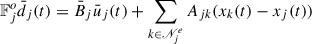 , and
, and  denotes the unknown inputs of the UIOi, j.
(2) The pair ( ) is detectable, where
 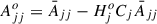 and
and 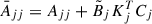 .
.
Then, decompose  into
into 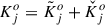 and determine the UIOi, j gain matrices
  ,
,  ,
,  , and
, and  based on the following conditions:
 (8a)
(8a)
 (8b)
(8b)
 (8c)
(8c)
 (8d)
(8d)
where I
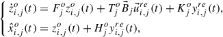
j ∈ ℝ3 × 3 is the identity matrix. The estimation error of UIOi, j is defined as  . Combining Equations (4), (7), and (8a)–(8d), yields its dynamics:
 (9)
(9)
It is evident that the estimation error  is independent of neighboring states; however, its complete decoupling from the disturbance
  and measurement noise
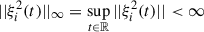
  has not yet been achieved. To improve the robustness of the UIOi, j, a performance output associated with
  is defined as
  . The designed observer gain is expected to ensure that the error system described by Equation (9), with performance output
  , achieves global uniform ℒ∞ stability with a performance index γ
j, satisfying the following conditions [22].
, achieves global uniform ℒ∞ stability with a performance index γ
j, satisfying the following conditions [22].
(1) The zero-input dynamics of the system Equation (9) (with  ) exhibits global uniform exponential stability concerning the origin.
(2) Given an arbitrary initial condition  and bounded exogenous input
  ,
,  , and
, and  , a finite bound
  can be determined such that
 (10)
(10)
(3) Given zero initial condition  and bounded exogenous input
  ,
,  , and
, and  , the following holds:
 (11)
(11)
(4) Given an arbitrary initial condition  and bounded exogenous input
  ,
,  , and
, and  , the following holds:
 (12)
(12)
To ensure that the UIOi, j achieves the desired ℒ∞ performance, the following theorem presents the conditions that its gain needs to satisfy, along with the method for solving the observer gain.
For the monitoring center of DGU i with UIOi, j Equation (7), providing observer gains  ,
,  ,
,  , and
, and  satisfy conditions Equations (8a)–(8d), and there exist matrix
  ,
,  and
and  , positive scalar α
j
o > 0, ν
j
1 > 0, and ν
j
2 > 0 such that the following inequality holds:
, positive scalar α
j
o > 0, ν
j
1 > 0, and ν
j
2 > 0 such that the following inequality holds:
![Mathematical equation: $$ \begin{aligned} \Upsilon _{j}^{o}&= \left[ \begin{array}{cccc} \bar{\Upsilon }_{j}^{o}&P_{j}^{o}&-S_{j}^{o}&P_{j}^{o}\\ *&-2\alpha _j^o\nu _j^1I_{j}&0&0\\ *&*&-2\alpha _j^o\nu _j^1I_{j}&0\\ *&*&*&-2\alpha _j^o\nu _j^1I_{j} \end{array} \right] \le 0, \end{aligned} $$](/articles/sands/full_html/2025/01/sands20250008/sands20250008-eq87.gif) (13)
(13)
![Mathematical equation: $$ \begin{aligned} \Psi _{j}^{0}&= \left[ \begin{array}{cc} P_{j}^{o}&C_{j}^T\\ *&\nu _j^2I_{j} \end{array} \right] \ge 0, \end{aligned} $$](/articles/sands/full_html/2025/01/sands20250008/sands20250008-eq88.gif) (14)
(14)
where  , then the estimation error dynamics Equation (9) of the UIOi, j is globally uniformly ℒ∞ stable with a performance index
  and observer gain
  .
.
Define a Lyapunov function as follows:
 (15)
(15)
Let  and
and  denote the maximum and minimum eigenvalues of
  , respectively. Then, from Equation (15), we have
 (16)
(16)
The time derivative of V j o(t) is given by
 (17)
(17)
Define ![Mathematical equation: $ \eta_j^o(t)=[e_{i,j}^{o}(t)^T, \xi_{j}^{1}(t)^T{T_{j}^{o}}^T, \xi_{j}^{2}(t)^T, -\dot{\xi}_{j}^{2}(t)^T{H_{j}^{o}}^T] $](/articles/sands/full_html/2025/01/sands20250008/sands20250008-eq98.gif) , one obtains
, one obtains
 (18)
(18)
where
![Mathematical equation: $$ \begin{aligned} \Omega _{j}^{o} = \left[ \begin{array}{cccc} \bar{\Omega }_{j}^{o}&P_{j}^{o}&-P_{j}^{o}\tilde{K}_{j}^{o}&P_{j}^{o}\\ *&-2\alpha _j^o\nu _j^1I_{j}&0&0\\ *&*&-2\alpha _j^o\nu _j^1I_{j}&0\\ *&*&*&-2\alpha _j^o\nu _j^1I_{j} \end{array} \right], \end{aligned} $$](/articles/sands/full_html/2025/01/sands20250008/sands20250008-eq100.gif) (19)
(19)
and  . Then, setting
  and substituting it into Equations (18) and (19), one obtains
 (20)
(20)
Thus, the establishment of Equation (13) can ensure Equation (20) ≤ 0, one obtains
 (21)
(21)
which implies
 (22)
(22)
By combining inequalities Equations (16) and (22), it can be derived that
 (23)
(23)
Thus, the zero-input dynamics of the system Equation (9) (with  ) is global uniform exponential stability concerning the origin and condition Equation (10) is satisfied. Then, defining the following matrix
![Mathematical equation: $$ \begin{aligned} \Psi _{j}^{0} = \left[ \begin{array}{cc} P_{j}^{o}&C_{j}^T\\ *&\nu _j^2I_{j} \end{array} \right] \end{aligned} $$](/articles/sands/full_html/2025/01/sands20250008/sands20250008-eq108.gif) (24)
(24)
and inequality Equation (14) is satisfied. By the Schur complement lemma, it can be concluded that
 (25)
(25)
By multiplying both the left and right sides of Equation (25) by  and its transpose, respectively, we obtain
 (26)
(26)
which implies  , Combined with Equation (22), we obtain
 (27)
(27)
Thus, condition Equations (11) and (12) are satisfied. This completes the proof. ■
Based on Equations (8a)–(8d) and Theorem 1, it is evident that the gain of UIOi, j implemented in DGU i can be determined solely using local information, independent of global system data. This local computation capability ensures the scalability of our proposed monitoring framework. Notably, the designed observer maintains its functionality without requiring global redesign when a compromised DGU is removed or a new DGU is integrated into the microgrid system.
Under the aforementioned design structure, the detection residual is crafted as 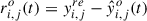 , where
 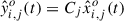 . The evaluation standard is determined by the Euclidean norm of residual
  . The detection mechanism functions according to the subsequent principle [5]:
 (28)
(28)
The detection mechanism in the control center of DGU i activates an alarm signal upon violation of the predetermined threshold boundary, indicating potential anomalies in communication link ij; conversely, the communication link ij is considered to be functioning normally. Notably, the threshold  is typically defined as
 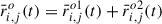 , where
  is a small constant introduced to reduce false alarms, and
  represents the supremum of residuals under attack-free conditions. While
  holds when the microgrid experiences no external disturbances and observer initialization matches the system’s initial state, these idealized assumptions rarely apply in practice. Thus, Monte Carlo simulations are conducted considering both measurement noise, load perturbations, and randomized initial conditions to statistically determine the residual supremum
  .
.
3.2. Implementation and analysis of collusive stealth attack
Considering the potential scenario where adversaries possess comprehensive knowledge of DGU models, they can design sophisticated attack signals to disrupt cyber-physical microgrid operations while evading detection. This section presents a systematic framework for constructing collusive stealth attacks, where the attacker simulates system dynamics to generate malicious signals. These signals are subsequently injected into the communication channel ij, concurrently compromising both the measurement y
j(t) and control input  . The measurement signal
  received by the control center of DGU i is expressed as in Equation (6), while the actual input signal
  is given by
  , where
  is dynamically generated as follows:
 (29)
(29)
where  represents the injected attack signal,
  and
and  are arbitrary non-zero false data. For simplicity, we denote
  . The following theorem demonstrates the stealthiness of the collusion attack strategy designed for communication link ij.
For the DC microgrids Equation (4) incorporating ℒ∞ UIO-based detection mechanisms Equations (7) and (28), the communication link ij is injected with  and y
i, j
a(t), where
and y
i, j
a(t), where  and y
i, j
a(t) are generated by Equation (29). This manipulation does not prompt an alert from the monitoring center, indicating that the collusion attack strategy is stealthy.
and y
i, j
a(t) are generated by Equation (29). This manipulation does not prompt an alert from the monitoring center, indicating that the collusion attack strategy is stealthy.
Considering  , the cyber-physical microgrid is free from malicious attacks and operates normally, the estimation error dynamics of the UIOi, j in the DGU i monitoring center is given by Equation (9). Considering
  , the communication link ij is subjected to the aforementioned collusion attack, the dynamics of the ℒ∞ UIOi, j can be expressed as follows:
 (30)
(30)
At this point, the detection residual can be expressed as:  , where
  . By integrating Equations (4), (8a)–(8d), (29), and (30), the dynamics of the estimation error can be derived:
 (31)
(31)
Evidently, the estimation error dynamics Equation (9) of the ℒ∞ UIOi, j in the absence of attacks are equivalent to those Equation (31) under the collusion attack, implying that the attack does not affect the detection residuals  , thereby maintaining stealthy. The proof is concluded. ■
The proposed collusive attack strategy simultaneously compromises the integrity of both y
j(t) and  . As evidenced by Equation (5), the corrupted measurement
  directly affects the secondary control input, consequently degrading system performance. Furthermore, Theorem 2 demonstrates that the error system dynamics remain consistent before and after the attack, indicating that the collusive attack does not induce residual anomalies. Consequently, this attack strategy can effectively disrupt system performance without triggering any alarm signals.
Compared to classical FDI attacks, the proposed collusion attack strategy exhibits enhanced destructiveness and stealthiness. Consequently, to ensure the continuous and stable operation of cyber-physical microgrids, it is imperative to devise corresponding countermeasures for timely detection of such malicious attacks.
4. Dynamic encoding detection scheme
In Theorem 2, it has been demonstrated that the proposed collusive attack is stealthy and can evade detection by the ℒ∞ UIO-based detection module. This section will present the design of a dynamic coding-based scheme to detect the aforementioned collusive stealthy attack. The core strategy involves integrating an encoder-decoder pair into the communication link ij to limit the adversary’s ability to disclose information. This ensures that the attacker cannot neutralize the system’s response through the injected signals  and y
i, j
a(t). As a consequence, the compromised measurement outputs
and y
i, j
a(t). As a consequence, the compromised measurement outputs  become discernible from the normal outputs y
j(t), causing the residual
become discernible from the normal outputs y
j(t), causing the residual  in the detection module to surpass the threshold
  significantly, thereby activating an alarm.
Actually, the control center of DGU i not only utilizes  to generate the secondary control input
  but also employs
  to estimate x
j(t), thereby monitoring anomalies in the communication link ij. As depicted in Figure 1, a pair of dynamic encoder and decoder is deployed in the communication link ij, where the input
to estimate x
j(t), thereby monitoring anomalies in the communication link ij. As depicted in Figure 1, a pair of dynamic encoder and decoder is deployed in the communication link ij, where the input  is encoded into
  before being transmitted over the communication network, with
  defined as follows:
 (32)
(32)
where Φ
j is an invertible matrix of appropriate dimension. Actually, the time-varying nature of e
cos(t)
Φ
j renders it inherently challenging for the attacker to accurately discern the coding matrix. Consequently, when a malicious adversary initiates the injection of attack signals  , unaware of the dynamic encoding scheme, the compromised signal is altered as follows:
 (33)
(33)
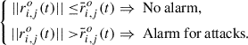
Before the input signal being transmitted into the control center,  undergoes decoding as follows:
 (34)
(34)
Evidently, the control signal of DGU i operates independently of  , ensuring that the aforementioned dynamic encoding mechanism does not interfere with the operation of the cyber-physical microgrid, thereby avoiding any degradation in system performance. On the other hand, in the absence of an attack scenario where
  , the input signal is restored to
 (35)
(35)
Consequently, the aforementioned dynamic encoding mechanism does not induce false alarms even in the attack-free scenario. The following theorem presents the estimation error dynamics of the UIOi, j in an attack scenario when the system employs the dynamic encoding mechanism.
In the DC microgrid Equation (4) equipped with the detection framework based on ℒ∞ UIO and dynamic encoding mechanism, the estimation error dynamics of UIOi, j when the collusive stealthy attack is injected into communication link ij can be represented as:
 (36)
(36)
That is, with the assistance of the dynamic encoding mechanism, the dynamics of the estimation error under collusive attacks differ from those under normal conditions, as described in Equation (36). By selecting appropriate dynamic encoding matrices, the detection residual  can be sufficiently amplified to exceed the predefined threshold
  , thereby triggering an alarm.
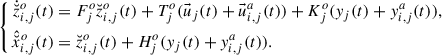
By combining Equations (4), (8a)–(8d), (29), (30), (34), and differentiating with respect to  , we obtain
 (37)
(37)
It is noteworthy that Equation (37) exhibits distinct characteristics compared to Equations (9) and (31). Specifically, the implementation of the dynamic encoding scheme alters the estimation error dynamics in the presence of collusive attacks. Given the relationship  , the residual undergoes corresponding variations, thereby depriving the collusive attack of its concealment. ■
Based on the above analysis, it is evident that when the system is not under attack, the dynamic encoding mechanism does not alter the normal control signals, unlike additive watermarking schemes, which modify control signals and consequently lead to system performance degradation. However, when the system is under attack, the collusive stealth attack loses its stealthiness due to the dynamic encoding mechanism, thereby triggering an alarm. To ensure the impact of the attack signal manifests in the residual signal  , the following theorem presents the feasibility conditions for the dynamic encoding matrix.
Based on the deployed ℒ∞ UIOi, j Equation (7) and dynamic encoding mechanism, the collusive stealthy attack Equation (29) can influence the detection residual  provided that the matrix
  possesses no non-minimum phase zero dynamics and
  , where
![Mathematical equation: $$ \begin{aligned} \mathbb{M} _{i,j}^{o}(s) = \left[ \begin{array}{cc} sI_j-F_j^o&T_{j}^{o}\vec{B}_{j}\Phi _j^{-1}E_{j}^{o}\\ C_j&0 \end{array} \right]. \end{aligned} $$](/articles/sands/full_html/2025/01/sands20250008/sands20250008-eq176.gif) (38)
(38)
Based on the analysis mentioned above, it can be concluded that after the implementation of the dynamic encoding mechanism, the error dynamics and detection residuals of UIOi, j are as follows:
 (39)
(39)
To ensure that the influence of any non-zero  on
on  is reflected in
  , it is necessary to select an appropriate encoding matrix such that the Rosenbrock system matrix
  possesses no non-minimum phase zero dynamics and is left-invertible, where
![Mathematical equation: $$ \begin{aligned} \tilde{\mathbb{M} }_{i,j}^{o}(s) = \left[ \begin{array}{cc} sI_j-F_j^o&e^{-\cos {(t)}}T_{j}^{o}\vec{B}_{j}\Phi _j^{-1}E_{j}^{o}\\ C_j&0 \end{array} \right]. \end{aligned} $$](/articles/sands/full_html/2025/01/sands20250008/sands20250008-eq182.gif) (40)
(40)
Moreover, since  , this condition is equivalent to require that the matrix
  possesses no non-minimum phase zero dynamics and is left-invertible. The left invertibility of the matrix
  is equivalent to the condition that the largest controllability subspace of system
  is contained within Ker(C
j), with
is contained within Ker(C
j), with  defined as zero. Furthermore,
  can be expressed as:
 (41)
(41)
where  represents the smallest conditioned invariant subspace encompassing
  , and
, and  denotes the largest weakly unobservable subspace. The computational procedure for determining these subspaces is outlined as follows [23, 24]:
 (42)
(42)
 (43)
(43)
where  and
and  converge to
  and
and  , respectively. Therefore, combining Equations (41)–(43), it can be concluded that when
  , then
  . This merely requires that
  does not lie in the null space of C
j, i.e.,
does not lie in the null space of C
j, i.e.,  . The proof is thus completed. ■
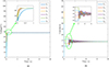 |
Figure 2. Simulation results under normal operating conditions. (a) and (b) correspond to the voltage at the PCC and the output current of the DGUs, respectively. |
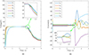 |
Figure 3. Simulation results under the scenario of the cyber-physical microgrid being subjected to the collusive stealthy attack. (a) and (b) correspond to the voltage at the PCC and the output current of the DGUs, respectively. |
5. Simulation results
To validate both the concealment and disruptive potential of the proposed coordinated attack strategy, along with the efficacy of the dynamic encryption-based detection mechanism, we implement a comprehensive simulation environment using the SimPowerSystems platform. The experimental setup encompasses a six DGUs microgrid configuration, with detailed electrical specifications and network topology referenced from [25].
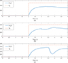 |
Figure 4. The detection threshold and detection residuals in the ℒ∞ UIO-based detection module. (a), (b) and (c) present the experimental results corresponding to UIO4, 2, UIO4, 3, and UIO4, 5, respectively |
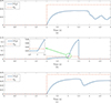 |
Figure 5. The detection threshold and detection residuals in the ℒ∞ UIO-based detection module with the deployment of the dynamic encoding mechanism. (a), (b) and (c) present the experimental results corresponding to UIO4, 2, UIO4, 3, and UIO4, 5, respectively |
Case 1: In this case, a simulation period of 20 s is considered, during which the cyber-physical microgrid operates without being subjected to any attacks. Initially, the six DGUs operate independently, with only the primary controller in effect. As shown in Figure 2a, the PCC voltages V
i rapidly track and stabilize at the reference values. At t = 2 s, the DGUs are interconnected via power lines, and the secondary controller is activated with current proportional parameter I
ti
s = 1, ∀i ∈ 𝒱p. As illustrated in Figure 2b, after a certain period of secondary controller operation,  is achieved, demonstrating that current sharing is realized in the cyber-physical microgrid under a reliable network environment.
Case 2: In this case, the simulation period is set to 5 s. Similarly, for the first 2 s, the DGUs are considered to operate independently, and they begin to interconnect at t = 2 s. At t = 3 s, the communication link among DGUs 2–4 is subjected to the collusive stealthy attack, where ![Mathematical equation: $ \vec{d}_{4,3}^a(t)=[0;0.1] $](/articles/sands/full_html/2025/01/sands20250008/sands20250008-eq205.gif) and y
4, 3
a(t) is generated by Equation (29). As shown in Figure 3, after the attack occurs, the voltage at the PCC fails to track the reference value and diverges. The current also exhibits significant oscillations, and
and y
4, 3
a(t) is generated by Equation (29). As shown in Figure 3, after the attack occurs, the voltage at the PCC fails to track the reference value and diverges. The current also exhibits significant oscillations, and  . This indicates that the negative impact of an attack on a single communication link rapidly propagates throughout the entire grid, affecting the overall system performance. Additionally, the monitoring results of UIO4, 2, UIO4, 3, and UIO4, 5 deployed in the DGU 4 are presented in Figure 4. After the attack, none of the detection residuals show noticeable anomalies, all remaining below the threshold. This demonstrates that the collusive attack successfully evades detection while degrading system performance, posing a significant threat to the microgrid.
Case 3: In this case, similar to Case 2, the communication network is subjected to the collusive stealthy attack. However, the dynamic encoding mechanism proposed in this paper is deployed in the communication network, and Φ 3 = [0.001, 0.05; 0, 0.001] is selected based on Theorem 4. The monitoring results of UIO4, 2, UIO4, 3, and UIO4, 5 in DGU 4 are shown in Figure 5. Before the attack occurs, all detection residuals remain below the threshold and exhibit no anomalies, indicating that the deployment of the dynamic encoding mechanism does not trigger false alarms. After the communication link among DGUs 2–4 is subjected to the collusive stealthy attack, the detection residual generated by UIO4, 3 exhibits an abnormal increase and quickly exceeds the threshold, while other detection residuals remain unaffected. This demonstrates that the proposed detection mechanism can accurately identify the attack and precisely locate the compromised link. At t = 3.5 s, DGU 3 is proactively disconnected to prevent further propagation of the attack effects. The remaining detection modules require no redesign and continue to monitor the microgrid effectively, highlighting the scalability of the proposed detection framework.
6. Conclusion
This paper has proposed a dynamic encoding-based detection framework to combat collusive stealthy attacks in cyber-physical microgrids. An ℒ∞ UIO was established at the control center to track communication link ij. The observer shows strong robustness, and its gain is calculated without needing information from neighboring DGUs. Subsequently, a collusive stealthy attack strategy has been proposed, which simultaneously compromises the integrity of input and output data, thereby disrupting grid performance, such as voltage regulation and current sharing. To counter the threat of the collusive stealthy attack, a dynamic encoding-based detection scheme has been introduced. This scheme does not degrade system performance in the absence of attacks but assists the ℒ∞ UIO in generating anomalous detection residuals in the presence of attacks. Additionally, the feasibility conditions for the encoding matrix have been rigorously analyzed. Finally, the destructiveness of the attack and the effectiveness of the detection framework have been validated through MATLAB-based microgrid simulations. Future research could extend the proposed detection framework to cyber-physical microgrids with nonlinear loads, along with the development of data-driven detection strategies based solely on system measurements.
Acknowledgments
We would like to thank all editors and reviewers who helped to improve the paper.
Funding
This work was supported in part by the Foundation for Innovative Research Groups of the National Natural Science Foundation of China (Grant No. 62421004), and in part by the National Natural Science Foundation of China (Grant Nos. 62173218 and 62103254).
Conflicts of interest
The authors declare no conflicts of interest.
Data availability statement
The original data are available from corresponding authors upon reasonable request.
Author contribution statement
Zhihua Wu: Conceptualization, Methodology, Formal analysis, Software, Validation, Writing-review & editing. Chen Peng: Data curation, Writing-original draft, Conceptualization, Methodology, Software, Supervision. Engang Tian: Visualization, Investigation, Methodology, Supervision. Yajian Zhang: Validation, Methodology, Formal analysis, Supervision.
References
- Zhang K, Shi Y, Karnouskos S, et al. Advancements in industrial cyber-physical systems: An overview and perspectives. IEEE Trans Ind Inform 2023; 19: 716–29. [Google Scholar]
- Chae J, Lee S, Jang J, et al. A survey and perspective on industrial cyber-physical systems (ICPS): From ICPS to AI-augmented ICPS. IEEE Trans Ind Cyber-Phys Syst 2023; 1: 257–72. [Google Scholar]
- Leng J, Sha W, Wang B, et al. Industry 5.0: Prospect and retrospect. J Manuf Syst 2022; 65: 279–95. [CrossRef] [Google Scholar]
- Peng C, Sun H, Yang M, et al. A survey on security communication and control for smart grids under malicious cyber attacks. IEEE Trans Syst Man Cybern: Syst 2019; 49: 1554–569. [Google Scholar]
- Ding SX. A note on diagnosis and performance degradation detection in automatic control systems towards functional safety and cyber security. Secur Saf 2022; 1: 2022004. [Google Scholar]
- Gao S, Zhang H, Wang Z, et al. Optimal injection attack strategy for cyber-physical systems: A dynamic feedback approach. Secur Saf 2022; 1: 2022005. [Google Scholar]
- Zhu K, Wang Z, Ding D, et al. Privacy-preserving control for 2-D systems with guaranteed probability. IEEE Trans Syst Man Cybern: Syst 2024; 54: 4999–5011. [Google Scholar]
- Liang G, Weller SR, Zhao J, et al. The 2015 Ukraine blackout: Implications for false data injection attacks. IEEE Trans Power Syst 2017; 32: 3317–318. [CrossRef] [Google Scholar]
- Condliffe J. Ukraine’s power grid gets hacked again, a worrying sign for infrastructure attacks. MIT Technology Review, 2016. [Google Scholar]
- Yang H, Yu Z, Zhang Y. Event-triggered resilient consensus control of multiple unmanned systems against periodic DoS attacks based on state predictor. Secur Saf 2023; 2: 2023017. [Google Scholar]
- Zhang Y, Mei D, Xu Y, et al. Adaptive cooperative secure control of networked multiple unmanned systems under FDI attacks. Secur Saf 2023; 2: 2023029. [Google Scholar]
- Qin J, Li M, Shi L, et al. Optimal denial-of-service attack scheduling with energy constraint over packet-dropping networks. IEEE Trans Automat Control 2018; 63: 1648–663. [Google Scholar]
- Tian E, Fan M, Ma L, et al. Stochastic important-data-based attack power allocation against remote state estimation in sensor networks. IEEE Trans Automat Control 2025; 70: 2012–019. [Google Scholar]
- Liu MX, Zhao CC, Deng RL, et al. False data injection attacks and the distributed countermeasure in DC microgrids. IEEE Trans Control Network Syst 2022; 9: 1962–974. [Google Scholar]
- Manandhar K, Cao X, Hu F, et al. Detection of faults and attacks including false data injection attack in smart grid using Kalman filter. IEEE Trans Control Network Syst 2014; 1: 370–79. [Google Scholar]
- Wang X, Luo X, Zhang M, et al. Detection and isolation of false data injection attacks in smart grid via unknown input interval observer. IEEE Internet Things J 2020; 7: 3214–229. [Google Scholar]
- Ye D, Zhang TY. Summation detector for false data-injection attack in cyber-physical systems. IEEE Trans Cybern 2020; 50: 2338–345. [Google Scholar]
- Esmalifalak M, Liu L, Nguyen N, et al. Detecting stealthy false data injection using machine learning in smart grid. IEEE Syst J 2017; 11: 1644–652. [Google Scholar]
- Farajzadeh-Zanjani M, Hallaji E, Razavi-Far R, et al. Adversarial semi-supervised learning for diagnosing faults and attacks in power grids. IEEE Trans Smart Grid 2021; 12: 3468–478. [Google Scholar]
- Wang X, Luo X, Zhang M, et al. Detection and isolation of false data injection attacks in smart grid via unknown input interval observer. IEEE Internet Things J 2020; 7: 3214–229. [Google Scholar]
- Gallo AJ, Turan MS, Boem F, et al. A distributed cyber-attack detection scheme with application to DC microgrids. IEEE Trans Automat Control 2020; 65: 3800–815. [Google Scholar]
- Xu B, Peng C, Zhang Y, et al. Distributed plug-and-play robust ℒ∞ voltage control for islanded microgrids. IEEE Trans Smart Grid 2024; 16: 1790–800. [Google Scholar]
- Trentelman HL, Stoorvogel AA, Hautus M, et al. Control theory for linear systems. London: Springer, 2012. [Google Scholar]
- Taheri M, Khorasani K, Shames I, et al. Cyberattack and machine-induced fault detection and isolation methodologies for cyber-physical systems. IEEE Trans Control Syst Technol 2023; 32: 502–17. [Google Scholar]
- Tucci M, Meng L, Guerrero JM, et al. Stable current sharing and voltage balancing in DC microgrids: A consensus-based secondary control layer. Automatica 2018; 95: 1–13. [CrossRef] [Google Scholar]

Zhihua Wu received the M.Sc. degree in operations research and cybernetics from the University of Shanghai for Science and Technology, Shanghai, China, in 2023. He is currently pursuing his Ph.D. degree in Control Science and Engineering at Shanghai University, Shanghai, China. His research interests include distributed control systems and smart grids.

Chen Peng (Senior Member, IEEE) received the B.Sc. and M.Sc. degrees in coal preparation and the Ph.D. degree in control theory and control engineering from the Chinese University of Mining Technology, Xuzhou, China, in 1996, 1999, and 2002, respectively. From November 2004 to January 2005, he was a Research Associate with the University of Hong Kong. From July 2006 to August 2007, he was a Visiting Scholar with the Queensland University of Technology, Brisbane, QLD, Australia. From July 2011 to August 2012, he was a Postdoctoral Research Fellow with Central Queensland University, Rockhampton, QLD, Australia. In 2012, he was appointed as an Eastern Scholar with the Municipal Commission of Education, Shanghai, China, and joined Shanghai University, Shanghai. His current research interests include networked control systems, distributed control systems, smart grids, and intelligent control systems.

Engang Tian (Senior Member, IEEE) received the B.Sc. degree in mathematics from Shandong Normal University, Jinan, China, in 2002, the M.Sc. degree in operations research and cybernetics from Nanjing Normal University, Nanjing, China, in 2005, and the Ph.D. degree in control theory and control engineering from Donghua University, Shanghai, China, in 2008. From 2011 to 2012, he was a Postdoctoral Research Fellow with the Hong Kong Polytechnic University. From 2015 to 2016, he was a Visiting Scholar with the Department of Information Systems and Computing, Brunel University London, Uxbridge, U.K. From 2008 to 2018, he was an associate professor and then a professor with the School of Electrical and Automation Engineering, Nanjing Normal University. In 2018, he was appointed as an Eastern Scholar by the Municipal Commission of Education, Shanghai, China, and joined the University of Shanghai for Science and Technology, Shanghai, China. He is currently a professor with the School of Optical-Electrical and Computer Engineering, University of Shanghai for Science and Technology, Shanghai. His research interests include networked control systems, as well as nonlinear stochastic control and filtering.

Yajian Zhang received the B.Sc. and M.Sc. degrees in electrical engineering from the China University of Mining and Technology in 2013 and 2016, respectively, and the Ph.D. degree in electrical engineering from Tianjin University, Tianjin, China, in 2021. He was a Postdoctoral Research Fellow in control theory and engineering with Shanghai University, Shanghai, China. Since 2024, he has been an associate professor at Shanghai University. His current research interests include secure networked control systems, power systems, cyber-physical systems, and power grid security control.
All Figures
|
Figure 1. The overall architecture diagram of cyber-physical microgrid |
| In the text | |
|
Figure 2. Simulation results under normal operating conditions. (a) and (b) correspond to the voltage at the PCC and the output current of the DGUs, respectively. |
| In the text | |
|
Figure 3. Simulation results under the scenario of the cyber-physical microgrid being subjected to the collusive stealthy attack. (a) and (b) correspond to the voltage at the PCC and the output current of the DGUs, respectively. |
| In the text | |
|
Figure 4. The detection threshold and detection residuals in the ℒ∞ UIO-based detection module. (a), (b) and (c) present the experimental results corresponding to UIO4, 2, UIO4, 3, and UIO4, 5, respectively |
| In the text | |
|
Figure 5. The detection threshold and detection residuals in the ℒ∞ UIO-based detection module with the deployment of the dynamic encoding mechanism. (a), (b) and (c) present the experimental results corresponding to UIO4, 2, UIO4, 3, and UIO4, 5, respectively |
| In the text | |
Current usage metrics show cumulative count of Article Views (full-text article views including HTML views, PDF and ePub downloads, according to the available data) and Abstracts Views on Vision4Press platform.
Data correspond to usage on the plateform after 2015. The current usage metrics is available 48-96 hours after online publication and is updated daily on week days.
Initial download of the metrics may take a while.