| Issue |
Security and Safety
Volume 4, 2025
Security and Safety in Artificial Intelligence
|
|
|---|---|---|
| Article Number | 2024025 | |
| Number of page(s) | 15 | |
| Section | Other Fields | |
| DOI | https://doi.org/10.1051/sands/2024025 | |
| Published online | 22 July 2025 | |
Research Article
Enhanlcing the accuracy of intrusion detection systems by reducing the rates of false negatives through using XG-boost and optimization algorithm
1
Department of Information and Communication Technologies, National School of Engineers of Tunis (ENIT), University of Tunis El-Manar, Tunis, 1008, Tunisia
2
Department of Cyber Security, College of Computer Science and Mathematics, Tikrit University, Tikrit, 3400, Iraq
3
Department of Computer Science and Mathematics, National Institute of Applied Sciences and Technology, Tunis, 1080, Tunisia
4
Department of Petroleum Project Management, College of Industrial Management of Oil and Gas, Basrah University for Oil and Gas, AI-Basrah, 61004, Iraq
* Corresponding authors (email: This email address is being protected from spambots. You need JavaScript enabled to view it.
)
Received:
26
July
2024
Revised:
5
November
2024
Accepted:
31
December
2024
Abstract
Intrusion Detection Systems (IDSs) are critical for network security, detecting and mitigating malicious activities. A key challenge in IDS implementation is the high rate of false negatives, where attacks go undetected, posing significant security risks. This study proposes an enhanced IDS model that integrates XG-boost, a robust gradient boosting algorithm, with Cat Swarm Optimization (CSO) to reduce false negatives and improve detection accuracy. XG-boost’s scalability and performance make it ideal for managing complex network traffic data, while CSO optimizes XG-boost’s hyperparameters by mimicking natural cat behaviors, ensuring optimal model performance. The proposed approach was evaluated using a benchmark dataset, demonstrating a notable reduction in false negatives compared to traditional IDS methods. The upgraded IDS also improve detection accuracy across various types of cyberattacks while maintaining a low false positive rate, crucial for minimizing disruptions to regular network operations. The optimized XG-boost model achieved an accuracy of 98%, with precision of 97.8% and an F1-score of 97.7%, significantly outperforming the non-optimized model (accuracy: 84.1%, precision: 86.5%, F1-score: 84.1%). These results highlight the effectiveness of the proposed method in real-world IDS deployment, where both security and operational efficiency are critical.
Key words: Catboost algorithm / Intrussion detection / Cyber security / XG-boost algorithm
Citation: Saud Abd N, Karoui K, and Ghassan Abdulkareem M. Enhanlcing the accuracy of intrusion detection systems by reducing the rates of false negatives through using XG-boost and optimization algorithm. Security and Safety 2025; 4: 2024025. https://doi.org/10.1051/sands/2024025
© The Author(s) 2025. Published by EDP Sciences and China Science Publishing & Media Ltd.
 This is an Open Access article distributed under the terms of the Creative Commons Attribution License (https://creativecommons.org/licenses/by/4.0), which permits unrestricted use, distribution, and reproduction in any medium, provided the original work is properly cited.
1. Introduction
Large volumes of data are now accessible in many different formats in our society due to emerging technologies, like cloud computing, social media, and big data analytics. Many security risks arise when we transmit such data over a network or internet. Although some cutting-edge intrusion prevention methods were developed to mitigate such risks, attacks nevertheless happen and keep getting bigger and bigger. We therefore need a dependable method for detecting any unauthorized traffic that could destroy the network [1]. More complex attacks than ever before are presently posing a challenge to network security due to the quick development of big data, the Internet, and AI. There is a growing need for network intrusion detection systems (NIDS) that are more potent and efficient. Related techniques are used by NIDS for collecting, cleaning, modelling, and identifying different types of network behaviors [2]. With the advancement of technology and the Internet, cyber-attacks are growing more frequent, which makes cyber security an essential element. On the Internet, there are many different kinds of attacks that might happen, such as denial of service (DoS), DNS spoofing, U2R (user-to-root), R2L (root-to-local), probe attacks, and more. Machine learning (ML) is a rapidly developing field that surpasses various legacy algorithms and encompasses a wide range of techniques. Cybersecurity professionals could utilize such techniques to find breaches [3, 4]. Artificial intelligence (AI) has become one of the most cost-effective and efficient approaches for constructing network intrusion detection systems (NIDS), as evidenced by its increasing popularity in recent years. A variety of machine learning (ML) and deep learning (DL) techniques are employed to develop models capable of distinguishing between normal data packets and intrusions, utilizing diverse methodologies to achieve this goal. In this study, we apply ML to extract meaningful information from the dataset and develop our NIDS model. Typically, several preprocessing techniques are employed in ML to select and clean the dataset before analysis. During this phase, missing values are addressed, and any errors in the dataset are corrected, ensuring a dataset free of errors. The dataset is then divided into two subsets: one for training and one for testing, with 80% typically used for training and 20% for testing [5]. After the training and testing phases are completed, the efficiency of the model can be evaluated. A variety of ML algorithms, such as decision trees, K-nearest neighbors, support vector machines (SVM), and K-means clustering, are commonly used to extract meaningful data from both raw and modified datasets. These algorithms have consistently demonstrated high efficiency in producing the desired outcomes.
The primary function of an intrusion detection system (IDS) is to monitor network traffic to identify unusual or suspicious activity and take preventive measures against potential intrusion threats. IDS systems are generally categorized into two types: network-based intrusion detection systems (NIDS) and host-based intrusion detection systems (HIDS). NIDS are typically deployed at key network points to monitor traffic that is more vulnerable to attack, while HIDS operates on specific devices connected to the network. Intrusion detection strategies are further classified into two main approaches: signature-based IDS and anomaly-based IDS [1, 6, 7]. Signature-based IDS focuses on identifying specific patterns, or “signatures”, of known intrusions and is regularly updated to account for emerging threats, including zero-day attacks. Anomaly-based IDS, also known as behavior-based detection, continuously monitors system activity and compares known behavioral patterns with new behaviors to identify potential threats. When an IDS alerts the system administrator, Intrusion Prevention Systems (IPS) can be used to mitigate threats such as Trojan horses and distributed denial-of-service (DDoS) attacks [2].
Developing an effective NIDS remains one of the most significant challenges in network security. Despite advances in NIDS technology, many current systems continue to rely predominantly on signature-based detection methods rather than anomaly-based protocols [3, 8]. Several factors contribute to the limited adoption of anomaly detection systems, including the dynamic nature of system behavior, the reliability and accuracy of training data, the collection of high-quality data, and the associated costs and error rates. These challenges can result in inaccurate and ineffective NIDS validation and solutions. Therefore, developing a more efficient intrusion detection system is crucial to addressing the limitations of current network security practices.
This research aims to minimize false negatives by developing an intrusion detection model through the application of multiple ML techniques to certain features acquired throughout the modelling stage. Since the false negative (FN) and false positive, (FP) rates are among the main issues with widely used procedures. FPs happen when the system misclassifies normal activity as harmful, while FNs happen in the case when the system fails to classify malicious behavior as such. Numerous actions are being conducted to tackle these issues. A sort of solution is provided by ML algorithms [9, 10]. ML algorithms search across a range of network activity datasets for appropriate hyper-parameters for classifiers to increase detection performance. Because they can handle missing values in data sets, incorporate techniques of regularization, optimize parallel as well as distributed computing, optimized tree pruning, and have a customizable objective function—all of which enable them to outperform other state-of-the-art and baseline ML algorithms—gradient boosting algorithms, like XG-boost, became more and more popular recently [11].
The intrusion detection framework consists of four modules: data collection, preprocessing, sampling, and production. Typical intrusion detection equipment. Data collection is important during the intrusion detection process. It is also crucial. Because the original security data is derived from numerous sources, there is heterogeneity, redundancy, and so on [5]. A direct analysis of the data will have a more detrimental impact. As a result, the preparation of raw data is crucial. Following preprocessing, the layer with the least amount of data is doubled in size, while the layer with the most data is reduced. Finally, the intrusion detection model will be trained and tested with the (XG-boost) approach. Then the results and confusion matrix were further enhanced using cat boost optimization [12].
We show similar work in Section 2. Section 3 describes the XG-boost Algorithms and then Cat Swarm Optimization in Section 4, while Section 5 describes the data that was used. A review of the research technique used in our work is presented in Section 6, including a section on the results. Lastly, we conclude our investigation in Section 7.
2. Related work
Numerous academics have attempted to address such performance concerns by utilizing IDS datasets and other ML techniques. In this study, we discussed some relevant research that merged different forms of optimization algorithms with the XG-boost algorithm for identifying attacks and producing good percentages as a consequence. We also looked into the false negative rates in some works, but the rates were slightly high and must be addressed.
-
Su P, Liu Y and Song X (2018) [5]. The intrusion detection model presented in this research is majorly based upon the XG-boost (Extreme Gradient Boosting), and it selects the necessary parameters using the Whale Optimization Algorithm (WOA). Before being inserted into the WOA-XG-boost algorithm, collected network data is pre-processed by using the PCA (i.e., Principal Component Analysis) dimensionality reduction technique, which improves data’s intrusion detection capabilities during training. The well-known KDD CUP99 data set from the field of computer networks is used to test the experimental findings. Additionally, the model of intrusion detection employed in this approach is more accurate in the case when put to comparison with the accuracy of discoveries made by adjusting the parameters in the prior method. WOA-XG-boost model is the most successful, according to the results. The method outperforms earlier algorithms in terms of sensitivity, specificity, and accuracy. With a sensitivity of 0.9958 and a specificity of 0.9574, the average ACC is 0.9906. The findings using Grid Search SVM were the most dismal. It demonstrates that for parameter optimization, the WOA approach performs better than the Grid Search methodology [5].
-
Bhattacharya S, Siva RS and Praveen KRM et al. (2020) [13]. This paper presents a hybrid firefly ML model for PCA that is intended to categorize IDS datasets. The research’s dataset was obtained from Kaggle. The model starts by applying one-hot encoding to alter IDS datasets. Dimensionality is subsequently decreased by using a hybrid PCA firefly approach. XG-boost algorithm is used to classify the reduced dataset. With the use of state-of-the-art ML approaches, they thoroughly evaluate the model to show the superiority of their suggested method. According to experimental results, the performance of the suggested model has been better than state-of-the-art ML models. They found that the specificity regarding XG-boost PCA, which had a slightly lower specificity score of 98.2%, was equivalent to that of plain XG-boost (99.9% specificity) and XG-boost PCA firefly (99.9% specificity). Regarding accuracy measurements, the results obtained from the three approaches are nearly identical. Nonetheless, the XG-boost-PCA-firefly method performs significantly better in terms of sensitivity than the other two algorithms (XG-boost 92.3%, XG-boost PCA 91.8%) [13].
-
Zivkovic M, Tair M and Venkatachalam K et al. (2022) [10]. This paper presents an enhanced version of the well-known Firefly method together with an application for modifying and optimizing the hyperparameters regarding the XG-boost classifier for network intrusion detection. The comparatively high false-positive and false-negative rates of NIDSs are one of the biggest causes for concern. The proposed study uses an improved Firefly approach to optimize the XG-boost classifier, resolving this issue. Before being contrasted with the original firefly method and other state-of-the-art metaheuristics, the suggested enhanced firefly algorithm was verified on 28 well-known CEC2013 benchmark examples utilizing methods from the current literature. After that, the proposed method was applied and assessed for XG-boost hyper-parameter optimization. The modified classifier was tested for network intrusion detection using the more recent USNW-NB15 dataset and the commonly utilized benchmarking dataset NSL-KDD. Based on experimental results, the suggested meta-heuristics have a great deal of promise for improving the accuracy of the classification as well as the average precision of the NIDSs, in addition to solving the ML hyperparameter optimization challenge [10].
-
Liu Z, Wang Y and Feng F et al. (2023) [1]. They have proposed an approach for the identification of the DDoS attacks in the SDNs combining feature engineering with Machine Learning. After CSE-CIC-IDS 2018 data-set cleaning and normalization, an enhanced binary grey wolf optimization algorithm was utilized to identify the best feature subset. The optimal DDoS attack detection classifier was selected after that and installed in the SDN controller after the ideal feature sub-set had been trained and then assessed in ML algorithms Random Forest (RF), Support Vector Machine (SVM), Decision Tree, K-Nearest Neighbor (k-NN), and XG-boost. According to the results, RF outperforms other models in several performance parameters, including precision, accuracy, F1, recall, and AUC values. They also investigate how various models and algorithms compare to one another. The findings demonstrate that while the F1-score and precision of RF (96), SVM (98), XG-boost (96), KNN (96), and decision tree (95) vary, there is a FN ratio of roughly 5% from dataset samples [1].
-
Cheng P, Xu K and Li S et al. (2022) [14]. Using a wrapper strategy that is based on a genetic algorithm for feature selection in network intrusion detection systems, Jaw and Wang offered an all-encompassing approach to intrusion detection systems. This approach allows for the selection of features in intrusion detection systems. Additionally, the use of logistic regression was utilized to accomplish ensemble learning. Their experimental findings on the CICIDS2017, NSL-KDD, and UNSW-NB15 datasets exhibited remarkable accuracy rates of 98.99%, 98.73%, and 97.997%, respectively. Additionally, their detection rates were 98.75%, 96.64%, and 98.93%, respectively. These results were derived from experiments in which just 11, 8, and 13 key characteristics were chosen from the datasets to arrive at the conclusions.
-
Gupta N, Jindal V and Bedi P (2022) [15]. To address the issue of class imbalance, Gupta et al. [15] suggested that network-based intrusion detection systems benefit from the implementation of ensemble approaches. Their method consisted of three stages: first, a deep neural network was utilized to differentiate between normal and suspect network traffic; second, eXtreme Gradient Boosting was utilized to identify large-scale attacks; and third, Random Forest was utilized to categorize less severe attacks. Although the time complexity was evaluated in hours rather than minutes, this model was able to attain accuracy rates of 99%, 96%, and 92%, respectively, when it was applied to the NSL-KDD, CIDDS-001, and CICIDS2017 datasets.
-
Tama BA and Lim S (2021) [16]. Two phases of ensemble learning classifiers were incorporated into the hybrid feature selection technique that was implemented by Tama BA and Lim S [16]. Their system was evaluated using the CIC-IDS2017 dataset, which had 37 features, and it obtained an accuracy of 96.46% during the testing process.
-
Mhawi DN, Aldallal A and Hassan S (2022) [17]. They suggested a unique IDS method for handling imbalanced and high-dimensional traffic with minimal DR, using hybrid methods depending on the desired FS. To achieve the optimal subset concerning function correlation, a hybrid CFS FPA strategy utilizing a 30-feature sample and a hybrid ensemble learning technique has been suggested. The suggested system was able to manipulate and process conflicts that the previous work suffered from, like the (FNR, FAR, accuracy, and DR), by eliminating non-essential features as well as selecting just affected features using the suggested approach CFS_FPA through the combination of the correlation feature selection and forest penalized attribute. As a result, accuracy in the testing phase increased to 87% and FNR was 0.123. The proposed model’s final experimental results, with the use of the CICIDS-2017 data set, demonstrated 99.73% accuracy, 99.82% precision, 99.71% F-measure, 99.8% DR, and 0.004 FAR. Moreover, the suggested approach outperforms the previously suggested CFS–FPA–ensemble approach and the existing classification algorithms. This approach has the potential to provide a significant competitive edge in IDS business when compared with the alternative methods. As a result, offers greater robustness and high reliability while spotting intrusions and categorizing benign traffic.
The above papers contributed to the writing of this paper, adding my practical experience and improvements through my use of hybridizing XG-boost with one of the optimization algorithms (cat swarm) to reduce false negatives to a minimum, as described in the results section.
3. XG-boost algorithms
An ML system called XG-boost makes use of gradient-boosted decision trees (GBDT). The finest ML software for classification, regression, and ranking problems is the one, which also incorporates parallel tree boosting [18]. Regarding prediction accuracy, gradient boosting is widely acknowledged to be superior to RF. An ensemble model provides strong prediction accuracy since it consists of several DTs. Since the DT forecasts the residual error regarding the preceding DT, it learns the model and prevents overfitting. Categorical boosting (Cat-boost), extreme gradient boosting (XG-boost), and light gradient boosting machine (LightGBM) are the three methods [19]. ML packages LightGBM, XG-boost, and Cat-boost have been based on the gradient boosting method. After being created in 2014, XG-boost has quickly become well-known as a result of its exceptional results on large data sets as well as multiple wins in the competitions of data science [18]. The main XG-boost objectives, incorporating the gradient-boosting DTs, are performance and speed. It represents a ma-chine augmentation method example that has been developed via Tianqi Chen and has since then been embraced by several developers. Through the prediction of the preceding DT’s residual error, DT avoids overfitting [20]. Gradient boosting-based Machine Learning libraries include LightGBM, XG-boost, and Cat-boost. Since it was created in 2014, XG-boost has been well-known because of its remarkable performance on large data sets and numerous victories in competitions of data science [18]. XG-boost uses gradient-boosting decision trees with the primary goal of increasing performance and speed. Numerous developers have now adopted Tianqi Chen’s method of adding machine augmentation, or augmenting machines. XG-boost is built using algorithms based on trees. The tree techniques use the qualities of the dataset, also referred to as features or columns, and use such features as the internal or conditional nodes. The state at the root node determines whether the tree splits into edges or branches. Splitting is typically done to arrive at a choice. The leaf node is the branch’s terminal, which does not produce any additional edges [21]. XG-boost model utilizes an additive training approach for optimizing objective functions; hence, the result of one optimization stage influences the subsequent step’s optimization procedure. The objective function of the model is represented as [22]. Large datasets can be effectively trained using scalable ML models, which is why scalability is appropriate. XG-boost is highly flexible because it has a wide range of hyper-parameters that may be changed to enhance performance. Missing Value Handling: Working with real-world data that commonly contains missing values is made easier by XG-boost’s built-in support to handle missing values. Interpretability: XG-boost places a strong emphasis on feature importance, making it easier to understand which factors to take into account when making predictions, unlike some ML algorithms that could be challenging to understand. Unfortunately, XG-boost is too computationally intensive for systems with limited resources, especially when training large models. An objective function is made up of a regularization term and a loss function is optimized via XG-boost. [23] defines the objective function.
 (1)
(1)
Θ denotes the model parameters for each tree in the ensemble.
n denotes the number of the training samples.
yi represents the true label of ith instance.
y ∧ i denotes the predicted value for ith instance.
L(yi, yi ∧) represents the loss function, which measures the difference between the predicted value and the true label.
K denotes the number of trees in the ensemble.
Ω(fk) denotes the regularization term applied to each tree in the ensemble.
Loss Function: The choice regarding loss function is based on the type of problem being solved. Common loss functions include:
Regression: Mean Squared Error (MSE).
Binary Classification: Binary Logistic Loss (logistic regression).
Multiclass Classification: Softmax Cross-Entropy
Regularization Term: XG-boost supports both L1 (Lasso) and L2 (Ridge) regularization terms to prevent overfitting. The regularization term is applied to each tree and is defined as:
 (2)
(2)
T denotes the number of leaves in a tree fk.
4. Cat swarm optimization
Yahoo created Cat-boost optimization (CSO) in the year 2017, and it is quite good at handling categorical variables. It is a better method that allows for quick learning on both GPU and CPU and automatically uses regularization to prevent overfitting [24]. Chu et al. (2006) and Tsai and Chu (2007) introduced CSO as a population-based and heuristic method for maintaining cats’ natural behavior. A cat’s innate desire to hunt is powerful. To find the optimal solution to a complex optimization problem, two sub-modes are being mathematically modelled [25]. In the case when they are resting, cats move very slowly and are constantly alert. We call this type of behavior “seeking mode”. Cats are quite aggressive and swift when they detect the presence of a bird. The term “tracing mode” refers to this mode [1]. There are 2 operation modes for the CSO algorithm, which are: seeking and tracing. A solution set has been represented by every cat, which has its own fitness value, position, and flag. The position in search space consists of M dimensions, every one of which has a different velocity; the flag indicates whether cats are seeking or tracing; the fitness value indicates how well the solution set (i.e., the cat) performs. Therefore, before we can run cats through the algorithm, we must first decide the number of cats that should be included in the iteration. The best cat from every one of the iterations is retained in memory, and the optimal solution is represented by the cat from the last iteration [16]. The six steps that make up the CSO process are as follows [26, 27]:
-
(1)
Set lower and upper boundaries for solution sets.
-
(2)
N cats (solution sets) should be randomly generated and distributed over an M-dimensional space, every one of which has a random velocity value that should not exceed the maximum velocity value that has been defined.
-
(3)
Sort the cats into tracing and seeking modes at random based on MR. A mixture ratio, or MR, is selected within the range [0, 1]. For instance, if N = 10 and MR = 0.2, then a random selection of 8 cats will enter the seeking mode, while the remaining 2 cats will enter the tracing mode.
-
(4)
All cats’ fitness values can be determined by using a domain-specific fitness function. After that, the best cat is selected and retained in memory.
-
(5)
After that, cats switch to tracing or seeking mode.
-
(6)
Divide the cats into seeking and tracing groups at random for the following iteration based on MR.
-
(7)
Check to see if the condition of termination is met; if not, restart Steps 4–6 and end the program.
4.1. Seeking mode
Four key parameters—counts of dimension to change (CDC), seeking memory pool (SMP), seeking a range of selected dimensions (SRD), and self-position considering (SPC)—have significant impacts on the seeking mode, which mimics the resting behavior of the cats. The user uses trial and error to fine-tune and define each of these parameters. The seeking memory size for cats is determined by SMP, which also defines the number of candidate positions that every cat will choose to go to. For instance, if SMP is set to 5, after that each cat will generate five new random positions, one of which will be selected to be the cat’s next position. The other 2 parameters, which are SRD and CDC, will determine the way to randomize the new placements. The number of dimensions that should be changed is specified by CDC and falls between 0 and 1. For instance, if the CDC is set to the value of 0.20 and the search space consists of 5 dimensions, after that for every cat, four of the dimensions must be changed at random while the fifth dimension remains unchanged. SRD stands for mutative ratio for the chosen dimensions; that is, it indicates the degree of modification and mutation for the dimensions that the CDC chose. Last but not least, SPC is a Boolean value indicating whether a cat’s present location will be selected as a candidate position for the following iteration. Because the present position is regarded as one of them, for instance, in the case where the SPC flag is set to true, we must produce the (SMP1) number of candidates for each cat rather than the SMP number. The steps for seeking mode are as follows:
-
(1)
Making as many as SMP copies of Catk’s current position.
-
(2)
For each one of the copies, as many CDC dimensions are selected randomly to be mutated. In addition to that, subtract or add SRD values randomly from current values, which replace old positions can be seen in the following equation:
 (3)
(3)
In which Xjdold denotes the current position; Xjdnew denotes the next position; j represents the number of a cat d represents dimensions; and rand represents a random number in the [0, 1] interval.
-
(3)
Evaluation of fitness value (FS) for all candidate positions.
-
(4)
Based upon the probability, perform the selection of a candidate point to be the next position for the cat where the candidate points that have a higher value of the FS have a higher chance to be chosen as can be seen from Equation (3). Nonetheless, if all of the fitness values are equal, then all selecting probability of every one of the candidate points needs to be set to 1.
 (4)
(4)
If minimization is the objective, then FSb = FSmax; else, FSb = FSmin.
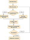 |
Figure 1. Cat swarm optimization algorithm general structure |
4.2. Tracing mode
This mode mimics how cats trace their surroundings. In the initial iteration, all of the cat’s position dimensions are assigned random velocity values. Yet, the values of velocity need to be changed for the following steps. The following are cats that move in this mode:
-
(1)
Update velocity values (Vk,d) for all dimensions based on Equation (5).
-
(2)
If a value of velocity outranged the maximum value, then it equals the maximum velocity value.
 (5)
(5)
-
(3)
Update Catk position based on the following equation:
 (6)
(6)
The Figure 1 shows the structure of the cat swarm optimization algorithm.
The feature engineering method in this study is enhanced by utilizing XG-boost’s capabilities to optimize data processing and model performance. Key techniques are included, such as handling missing values directly within the model, ensuring data integrity without extensive preprocessing, and focusing on feature importance for selecting impactful variables, which improves interpretability and accuracy. Performance is optimized, and overfitting is controlled through hyperparameter tuning, including adjustments to learning rates, maximum depth, and regularization terms (L1 and L2). Regularization techniques are applied to each tree in the ensemble, allowing a balance between complexity and generalizability. The objective function is optimized based on the problem type, with specific loss functions like Binary Logistic Loss being used for classification. Additionally, an iterative learning process is enabled by XG-boost’s tree-based structure and additive training approach, where each tree is adjusted based on previous residual errors, refining accuracy at each step. Through these methods, a scalable and interpretable solution ideal for constructing an effective network intrusion detection system is provided.
Advantages such as efficient handling of categorical variables and prevention of over-fitting are offered by Cat-boost optimization (CSO). However, several limitations are associated with it. First, parameters that require careful tuning (e.g., counts of dimension to change, seeking memory pool (SMP), and seeking a range of selected dimen-sions are relied upon by the CSO algorithm, making the process time-consuming and computationally expensive, particularly in high-dimensional datasets. Additionally, exploration of the solution space may be limited by the division of cats into seeking and tracing modes in CSO. The stochastic nature of CSO can also lead to variable results across runs, impacting consistency and model reliability. Moreover, the computational intensity of updating each cat’s velocity and position at every iteration, particularly for large datasets and complex optimization tasks, can be considerable. Lastly, although strengths are present, substantial resources and careful parameter management are re-quired by CSO, which can restrict its scalability and efficiency in certain applications. Finally, the basic steps of the model can be explained in general in Figure 2.
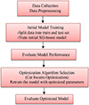 |
Figure 2. Model of the XG-boost and optimization algorithm |
5. Dataset
The present data contains different kinds of IoT intrusions. The categories of the IoT intrusions enlisted in the data are (DDoS, Spoofing, Brute Force, Web-based, Mirai, and DoS, Recon). The dataset contains 1191264 network intrusion incidents, each with 47 characteristics. The dataset can be used to develop a predictive model capable of detecting various types of invasive attacks. The data is also appropriate for designing the IDS system [28].
6. Methodology
6.1. Data preprocessing
The data contains a large number of classes with values that vary greatly, and the following Figure 3 shows the distribution of each one of them.
 |
Figure 3. The distribution of attack in the dataset |
Here, some scripts have code that has been used to convert the values in the Label column from a dataset to specific labels based on a specific mapping for each label. Since the attacks are not known in our data, so we will remove the label field by hearing this instruction:
data.drop(columns=[‘label’], inplace=True)
And create a new column “attack_category”. The code starts by creating a new column called “attack_category” in the DataFrame based on the attack categories mapping defined in attack_mapping. As shown in the following command:
data[‘attack_category’] = data[‘label’].apply(lambda x: next((category for category, attacks in attack_mapping.items() if x in attacks), x))
Printing the new distribution of attack categories:
Finally, the code prints out the distribution of values in the newly created ’attack_category’ column.
print(data[‘attack_category’].value_counts())
data[‘attack_category’].value_counts(): This function calculates the frequency of every one of the unique values in the ‘attack_category’ column and returns the counts as a Series. The print() statement then displays this Series, showing how many times each attack category appears in the dataset.
In summary, this code snippet performs a transformation on the ‘label’ column of a DataFrame (data) based on a predefined mapping (attack_mapping), creating a new ‘attack_category’ column with mapped values. It then removes the original ‘label’ column and prints out the distribution of attack categories in the dataset after the transformation.
As a result, some categories with very small sizes were included in the larger category, and the following Figure 4 shows the final results [29].
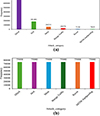 |
Figure 4. Frequency of attack catergory values before and after optimization: (a) before optimization; (b) after transmit it to be balanced |
The proposed approach, which combines XG-boost with Cat Swarm Optimization (CSO), outperforms the baseline XG-boost model and other existing IDS solutions with traditional parameter tuning methods like grid search or random search. While the baseline XG-boost model relies on default hyperparameters, leading to suboptimal performance, the CSO-based approach systematically searches for optimal hyperparameter values, improving model accuracy, precision, recall, and F1 score. Compared to traditional tuning methods, the proposed CSO method is more efficient, as it balances exploration and exploitation, avoiding local optima and reducing computational overhead. This results in better detection rates and fewer false positives, making the proposed approach particularly effective in intrusion detection tasks.
We noticed a very large imbalance between the classes in the data, therefore we solved the problem, and these are the results.
6.2. The result of optimizing XG-boost model with Cat Swarm optimization algorithm
Given the poor level of accuracy achieved by the first model XG-boost, and to increase the model’s efficiency in detecting threats, we hybridized the basic model with a modern improvement algorithm, according to the steps shown in the following diagram: These are the results that were achieved. Table 1 shows the measurements of models before and after optimization.
The measurements of models before and after optimization
Classification results of each attack before optimization
Classification results of each attack after optimization
Table 2 shows the classification values before optimization in detail for each attack in the dataset.
Table 3 shows the classification values after optimization in detail for each attack in the dataset.
As shown in Figure 5, the confusion matrix is also shown before and after optimization, where we notice a significant decrease in false negative values.
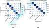 |
Figure 5. Confusion matrix of the model. (a) Confusion Matrix Before Optimization; (b) Confusion Matrix After Optimization |
We also show the confusion matrix for the result of our work in Figure 5.
We also show the receiver operating characteristic (ROC) curve of the models in Figure 6, where receiver operating characteristics (ROCs) are used to examine the relationship between correctly recognized target items (i.e., the hit rate) and incorrectly recognized lure items (i.e., the false alarm rate) across variations in response criterion.
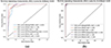 |
Figure 6. Receiver Operating Characteristic (ROC) curve for the models. (a) ROC of the model before optimization; (b) ROC of the model after optimization |
Figure 7 shows another design of the (ROC) curve showing the training and validation of the model.
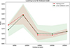 |
Figure 7. The ROC curve for the XG-boost model |
We also notice from the Receiver Operating Characteristic (ROC) curve how the model’s performance has improved and this is illustrated in Figures 5–7.
6.3. Summary of comparison
In conclusion, the CSO-XG-Boost approach generally outperforms the baseline XG-Boost and other IDS solutions in terms of performance, optimization efficiency, and handling imbalanced data. It strikes an optimal balance between computational complexity and detection accuracy, making it a robust and scalable choice for IDS tasks, as shown in Table 4.
Summary of comparison
7. Conclusion
For an ML model to effectively generalize and generate precise predictions across several classes, data balance is crucial. Biased models which perform well on the majority class, yet badly on the minority class could result from imbalanced data. To solve this, we employed oversampling in our research (see Figures 4a and 4b): increasing the number of cases in the minority class using methods such as SMOTE (Synthetic Minority Over-sampling Technique). Yet, there is not a one-size-fits-all approach to data balance. It necessitates giving the dataset, the current issue, and the selected model considerable thought. More fair, robust, and reliable ML models result from properly balanced data. However, algorithms have shown to be effective methods for resolving challenging optimization issues. They exhibit good research skills and take inspiration from natural phenomena. Those algorithms have been effectively used in many different sectors over the years, such as biology, logistics, engineering, and finance. Despite the considerable success that meta-heuristic algorithms have had, there are still issues and room for development. Combining two algorithms could enhance output and productivity. Here, we hybridized XG-boost algorithms with Cats-warm optimization to achieve high accuracy and precision with little FN. The results are displayed in the confusion matrix in Figure 5, Table 2 and Table 3.
Acknowledgments
The authors would like to acknowledge the Computer Science Department, Tikreet university and the National Institute of Applied Sciences and Technology, Tunisia.
Funding
This research received no specific grant from any funding agency in the public, commercial, or not-for-profit sectors.
Conflicts of interest
The authors declare no conflict of interest.
Data availability statement
Data are available upon request from the authors and also available on the Kaggle repository.
Author contribution statement
Noor Saud Abd: writing the original draft and conceptualization; Mohammed Ghassan Abdulkareem: writing, reviewing, editing and supervision; Kamel Karoui: supervision and methodology.
References
- Liu Z, Wang Y and Feng F et al. A DDoS detection method based on feature engineering and machine learning in software-defined networks. Sensors 2023; 23: 6176. [Google Scholar]
- Saied M, Guirguis S and Madbouly M. Review of artificial intelligence for enhancing intrusion detection in the internet of things. Eng Appl Artif Intell 2024; 127: 107231. [Google Scholar]
- Jiang H, He Z and Zhang H. Network intrusion detection based on PSO-XG-boost model. IEEE Access, 2020; 8: 58392–401. [Google Scholar]
- Aziz NAM, Yunus R and Abd Hamid H et al. An acceleration of microwave-assisted transesterification of palm oil-based methyl ester into trimethylolpropane ester. Sci Rep 2020; 10: 19652. [Google Scholar]
- Su P, Liu Y and Song X. Research on intrusion detection method based on improved smote and XG-boost. In: Proceedings of the 8th International Conference on Communication and Network Security, 2018. [Google Scholar]
- Abdulkareem-Alsultan G, Asikin-Mijan HV and Lee YH et al. Biofuels: past, present, future. Innovations Sustainable Energy Cleaner Environ 2020; 489–504. [Google Scholar]
- Kamil FH, Ali S and Shahruzzaman RMHR et al. Characterization and application of aluminum dross as catalyst in pyrolysis of waste cooking oil. Bull Chem React Eng Catal 2017; 12: 81–8. [Google Scholar]
- Abdulkareem-Alsultan G, Asikin-Mijan N and Obeas LK et al. In-situ operando and ex-situ study on light hydrocarbon-like-diesel and catalyst deactivation kinetic and mechanism study during deoxygenation of sludge oil. Chem Eng J 2022; 429: 132206. [Google Scholar]
- Venkatesan S, Design an intrusion detection system based on feature selection using ML algorithms. Math Stat Eng Appl 2023; 72: 702–10. [Google Scholar]
- Zivkovic M, Tair M and Venkatachalam K et al. Novel hybrid firefly algorithm: An application to enhance XG-boost tuning for intrusion detection classification. PeerJ Comput Sci 2022; 8: e956. [Google Scholar]
- Fuhnwi GS, Revelle M and Izurieta C. Improving network intrusion detection performance: an empirical evaluation using extreme gradient boosting (XG-boost) with recursive feature elimination. In: 2024 IEEE 3rd International Conference on AI in Cybersecurity (ICAIC). IEEE, 2024. [Google Scholar]
- Leevy J, Machine Learning Algorithms for Predicting Botnet Attacks in IoT Networks. 2022, Florida Atlantic University. [Google Scholar]
- Bhattacharya S, Siva RS and Praveen KRM et al. A novel PCA-firefly based XG-boost classification model for intrusion detection in networks using GPU. Electronics 2020; 9: 219. [Google Scholar]
- Cheng P, Xu K and Li S et al. TCAN-IDS: intrusion detection system for internet of vehicle using temporal convolutional attention network. Symmetry 2022; 14: 310. [Google Scholar]
- Gupta N, Jindal V and Bedi P. CSE-IDS: Using cost-sensitive deep learning and ensemble algorithms to handle class imbalance in network-based intrusion detection systems. Comput Secur 2022; 112: 102499. [Google Scholar]
- Tama BA and Lim S. Ensemble learning for intrusion detection systems: A systematic mapping study and cross-benchmark evaluation. Comput Sci Rev 2021; 39: 100357. [Google Scholar]
- Mhawi DN, Aldallal A and Hassan S. Advanced feature-selection-based hybrid ensemble learning algorithms for network intrusion detection systems. Symmetry. 2022; 14: 1461. [Google Scholar]
- Chen T and Guestrin C. XG-boost: A scalable tree boosting system. In: Proceedings of the 22nd ACM Sigkdd International Conference on Knowledge Discovery and Data Mining. 2016. [Google Scholar]
- Basheri M and Ragab M. Quantum cat swarm optimization based clustering with intrusion detection technique for future internet of things environment. Comput Syst Sci Eng 2023; 46: 3783. [Google Scholar]
- Ke G, Meng Q and Finley T et al. Lightgbm: A highly efficient gradient boosting decision tree. Adv Neural Inf Process Syst 2017; 30: 3146. [Google Scholar]
- AlHosni N, Jovanovic L and Antonijevic M et al. The XG-boost model for network intrusion detection boosted by enhanced sine cosine algorithm. In: International Conference on Image Processing and Capsule Networks. Springer, 2022. [Google Scholar]
- Dhaliwal SS, Nahid A-A and Abbas R. Effective intrusion detection system using XG-boost. Information 2018; 9: 149. [CrossRef] [Google Scholar]
- Wang J and Zhou S. CS-GA-XG-boost-based model for a radio-frequency power amplifier under different temperatures. Micromachines 2023; 14: 1673. [Google Scholar]
- Ihsan RR, Almufti SM and Ormani BMS et al. A survey on Cat Swarm Optimization algorithm. Asian J Res Comput Sci 2021; 10: 22–32. [Google Scholar]
- Seyyedabbasi A and Kiani F. Sand Cat swarm optimization: A nature-inspired algorithm to solve global optimization problems. Eng Comput 2023; 39: 2627–51. [Google Scholar]
- Chu SC, Tsai PW and Pan JS. Cat swarm optimization. In: PRICAI 2006: Trends in Artificial Intelligence: 9th Pacific Rim International Conference on Artificial Intelligence Guilin, China, August 7-11, 2006 Proceedings 9. Springer, 2006. [Google Scholar]
- Abdulraheem SA, Aliyu S and Abdullahi FB. Hyper-parameter tuning for support vector machine using an improved cat swarm optimization algorithm. J Nigerian Soc Phys Sci 2023; 5: 1007. [Google Scholar]
- Neto ECP, Dadkhah S and Ferreira R et al. CICIoT2023: A real-time dataset and benchmark for large-scale attacks in IoT environment. Sensors 2023; 23: 5941. [Google Scholar]
- Ahmed AM, Rashid TA and Saeed SAM. Cat swarm optimization algorithm: a survey and performance evaluation. Comput Intell Neurosci 2020; 2020: 4854895. [Google Scholar]

Noor Saud Abd has received the M.S. in computer science from Diyala University, Iraq, in 2021. Now, She is a lecturer at the department of cyber security from Tikrit University, Iraq. Her research interests are cyber security, machine learning, artificial intelligence, and data science.

Kamel Karoui currently works at the Computer Science & Maths, National Institute of Applied Sciences and Technology, Tunisia. Kamel does research in computer communications (networks), computer security and reliability and distributed computing.

Mohammed Ghassan Alsultan has received the M.S. in Computer and Communication Engineering from Islamic University of Lebanon, Lebanon, in 2021. He is a lecturer at the Department of oil and Gas Management and Marketing, College of Industrial Management of oil and Gas, Basra University for Oil and Gas, Al-Basrah, Iraq. His research interests are deep learning, computer vision, machine learning, artificial intelligence, pattern recognition, image processing, and biometrics.
All Tables
All Figures
|
Figure 1. Cat swarm optimization algorithm general structure |
| In the text | |
|
Figure 2. Model of the XG-boost and optimization algorithm |
| In the text | |
|
Figure 3. The distribution of attack in the dataset |
| In the text | |
|
Figure 4. Frequency of attack catergory values before and after optimization: (a) before optimization; (b) after transmit it to be balanced |
| In the text | |
|
Figure 5. Confusion matrix of the model. (a) Confusion Matrix Before Optimization; (b) Confusion Matrix After Optimization |
| In the text | |
|
Figure 6. Receiver Operating Characteristic (ROC) curve for the models. (a) ROC of the model before optimization; (b) ROC of the model after optimization |
| In the text | |
|
Figure 7. The ROC curve for the XG-boost model |
| In the text | |
Current usage metrics show cumulative count of Article Views (full-text article views including HTML views, PDF and ePub downloads, according to the available data) and Abstracts Views on Vision4Press platform.
Data correspond to usage on the plateform after 2015. The current usage metrics is available 48-96 hours after online publication and is updated daily on week days.
Initial download of the metrics may take a while.